17. ECONOMICS

17.1. Introduction into the Economics submodel and its main principles

The Economics submodel aims to capture socio-economic pressures that determine harvesting decisions. There is an increasing realisation that human behaviour and socio-economic drivers are important determinants of marine resource use, but many models do not attempt to capture this. To fill this gap, Atlantis includes Economics submodels. However, users should be aware that the Economics submodel has not been used and tested as widely used as other submodels (e.g. biology) and should be used with caution. When applying this submodel it is recommended to start with simple options, where model outputs against the expectations. In this manual only the key routines are described; users interested in further details should consult the key publications listed below, the Atlantis wiki, the Atlantis google groups or the Atlantis model developers.

NoteKey References: Economics Submodels in Atlantis

1. Kaplan IC, Holland DS, Fulton EA (2014) Finding the accelerator and brake in an individual quota fishery: linking ecology, economics, and fleet dynamics of US West Coast trawl fisheries. ICES Journal of Marine Science (Dan Holland economics model version, fish prices and quota trading)

2. van Putten EI, Gorton B, Fulton B, Thebaud O (2013) The role of behavioural flexibility in a whole of ecosystem model. ICES journal of Marine Science, 70(1), 150-163. doi:10.1093/icesjms/fss175 (fisher behaviour, flexibility and historical information use)

3. Hutton T, Thebaud O, Fulton B, Pascoe S, Innes J, Kulmala S, Tudman M (2010) Use of economic incentives to manage fisheries bycatch: An application to key sectors in Australia’s Southern and Eastern Scalefish and Shark Fisheries. Australian Fisheries Management Authority report (economic incentives to minimise bycatch and discards, deemed values, taxes on bycatch)

4. Fulton EA, Smith ADM, Smith DC (2007) Alternative management strategies for Southeast Australian Commonwealth fisheries. Australian Fisheries Management Authority and Fisheries Research and Development Corporation report

Original descriptions of quota trading models, now implemented in Atlantis

5. Little et al. (2009) An agent-based model for simulating trading of multi-species fisheries quota. Ecological Modelling 220, 3404–3412 — quota trading study implemented in Atlantis.

6. Newell RG, Sanchirico JN, Kerr S (2005) Fishing quota markets. Journal of Environ. Econ. Manag. 49: 437–462 — an alternative quota trading version implemented in Atlantis.

General principles of the Economics submodel

1. Fisheries are divided into subfleets to allow for differences in gear, costs, hold size, crew characteristics, home port distributions, targeting, quota holding, personal attitude profiles and travelling distances. This allows more flexible fishing effort dynamics.

2. Fishing effort is modelled through market dynamics, which means that fish prices and fishing costs vary through time, and fishers mostly distribute their effort to maximise profit.

3. Under a TAC system, quota can be traded dynamically among fishers. Unlike in non-economics based fisheries effort models, TACs may not be fulfilled (i.e. no, or not all quota will be used) if fishing is unprofitable such as when fish prices are low or fishing costs are high.

4. Some level of non profit maximising human behaviour is allowed. Many fisheries decisions in the real world are based on criteria other than profit maximisation (lifestyle, beliefs, habit). In Atlantis, this is implemented through an extra parameter defining the flexibility of fishers to learn and so change effort to match the areas of highest CPUE (see chapter 17.5), and by introducing stochasticity in gear switching, vessel update routines and quota trading routines (see chapters 17.3 and 17.4.1).

5. There is the potential to implement a quota trade network where for instance, there is preferential trading between fleets or subfleets. This can emulate empirically based or hypothetical preferential trading based on kinship, friendship, or business relationships. This is not activated in all versions of the code and anyone interested in using it should approach the Atlantis developers for support in its use.

6. The module outputs some simple economic indicators. However, these should be used with caution as the Atlantis developers are not economists and have not always used standard economics conventions with regard to terminology and the use of discount factors.

NoteWhat is a subfleet and why is it needed?

Subfleets are used to model fisher behaviour at a higher resolution, along the lines of metiers as defined by Pelletier et al (2000) or Deporte et al (2012). The idea is to divide up fishing fleets into subfleets (metiers) with similar properties. The key aspects of subfleets is that they can have different costs of fishing, behavioural flexibility and quotas. The subfleet behaviour is used to better reflect dynamic effort changes of different fisheries. The profits of fishing operations are also tracked at the subfleet level and dynamic changes in the numbers or activities of subfleets shapes the realised fishing practices at the fleet level.

Subfleets are only defined in the Economics submodel – in the Harvest submodel the actual catches are done at the level of fisheries, as described in chapter 15.4. This is to maximise compatibility with the other ways of representing fisheries. However, it also means that regardless of the vessel sizes or fishing costs, all subfleets within one fishery are characterised by the same gear selectivity, fish escapement, incidental mortality and other fishery specific parameters given in the dynamic fishing equations in chapter 15.4. The only thing that is affected by subfleets in the Harvest submodel is the effort per fishery per box per timestep.

The subdivision of fisheries into subfleets is used to have a more dynamic representation of effort allocation per box per time step. When the Economics submodel is used, effort allocation reflects fisher behaviour and subfleets can respond to markets and trade quota.

The Economics option is only available when dynamic fishing is used (so imposed catches or user defined fishing mortality do not have the option to turn on Economics).

Parameters in the economics.prm are mostly subfleet specific and include:

Number of boats, hold size, crew size, behaviour flexibility, costs of fishing, quota allocation

All fisheries related parameters defined in the harvest.prm file are identical among subfleets within a fishery, including:

Gear selectivity, target species, fish escapement, incidental mortality, discarding, minimum and maximum fishing depth, fishing habitat characteristics and so on

Parameter	Description
YYY_nsubfleets	Number of subfleets per each fishery. This value is only used if economics is switched on for that fishery. If the economics sub-model is being used then this value must be at least 1 or Atlantis will crash.
YYY_nlicence	Number of licences for each fishery across all subfleets. It defines the maximum number of vessels that may be active in a fishery.
YYY_nboat	Number of boats in each subfleet. The array should have as many entries as the maximum number of subfleets. For fisheries that have fewer or only 1 subfleet, give 0 for the remaining “empty” subfleets. For fisheries that have an effortmodel value < 12 then set all values to 0 (as they are not modelled using subfleets but instead use one of the effort models defined in the harvest sub-model).
YYY_boat_size	Boat size (m) for each subfleet.
YYY_hold_capacity	Hold capacity (in tonnes). Used in the Dan Holland effort allocation option.
YYY_crewsize	Number of full time equivalent people in the crew.
YYY_home_port	Port for each subfleet (with the number corresponding to the port numbers defined in the harvest.prm). This will be important when weighing the distance of boxes to ports in effort allocation.
YYY_triplength	Average length of a fishing trip (in days).
YYY_FishableLength	Length of time (hours per day) spent fishing.
YYY_ShotLength	Length of one fishing effort or shot (in hours) for each subfleet. This is used to calculate the final effort (in days per day) for each fishery.
YYY_MaxShotVol	The volume of one fishing effort or shot (in tonnes). This is only used in the shot-by-shot fine scale calculations and not in the general economics sub-model.
YYY_minDownTime	The proportion of the total time that each subfleet must stay in the port (for maintenance, etc.). This will decrease the maximum possible effort each subfleet can apply.
month_scalar	Global parameter setting up the scalar in number of days per month that each subfleet can apply. It is used in calculating max_month_effort, see chapter 17.
BycatchCountDiscards	This flag indicates whether the discard of bycatch species are used in calculations involving total catches (e.g. for calculating total catch per box vs profit or taxes, used in deciding where to target fishing effort). The inclusion of bycatch may be important if there are penalties or taxes for taking endangered species.

Table 15. General Economics and subfleet parameters

17.2. Key routines of the Economics submodel

If the Economics submodel is turned on (flagecon=1 in the run.prm file) the Economics() routine is called at every time step, setting up fishing dynamics based on sub-fleet parameters.

The key steps done in the Economics() routine are:

1. Allocate catch from the Harvest submodel to subfleets of each fishery. In the Harvest and Ecology submodels all catch is applied and recorded at the level of a fishery. In the Economics submodel, however, fisher behaviour and dynamic fishing is more resolved and modelled at the level of subfleets within each fishery. Once the harvest per species per age group per fishery per box is calculated in the Harvest submodel it is then passed back into the Economics submodel, where it is divided among subfleets. This allocation to subfleets is proportionally based on the effort for each subfleet in that cell in the previous time step (stored in the “black books” of each subfleet, see below) and the availability of quota for that subfleet. The allocation of catch among subfleets is done by the Allocate_Catch() routine ateconresponse.c.

2. Assess the economic situation or market behaviour, i.e. calculate fish prices (used in deciding what to fish), calculate quota prices (for quota trading) and a range of economic indicators. This is done in Get_Fish_Prices(), Total_Quota_Price() and Economic_Indicators() routines. The economic indicators are used for reporting purposes only and do not affect the simulations. See chapter 17.3 for further description.

3. At the start of the month assess the subfleet’s economic status and prospects, any responses to the market leading to buying or selling of boats, and update number of boats associated with ports and different markets. This is done in Update_Vessel_Numbers() and Port_Growth() routines. Subfleets can run at a loss (i.e. costs are greater than returns) for certain periods of time – and debts (negative profits) are created. If expected profit is not sufficient to reduce the debt levels and debts become ‘crippling’, after a certain amount of time a subfleet will start decreasing effort. A subfleet may exit the fishery (i.e. boats are decommissioned) if the debt is large and continues for too long. See chapter 17.4 for further description.

4. Make an annual (start of the year) and monthly (start of the each month) plan for fishing effort. Here fishers make decisions where and how much they are planning to fish. The plan is first made for the whole year based on the historical catches and profits (stored in “black books” of each subfleet) versus expected profit for this year (the profit expectation might change depending on the costs of fishing, prices of fish and quota availability) and flexibility of fishers to change their behaviour. The main routines for annual effort planning is Annual_Effort_Schedule() and Dynamic_Effort_Allocation() in atEconomicAnnual.c. Then each month the annual effort plan is updated depending on whether realised catches are close to expected catches and (how the fishery is tracking in terms of the ratio of realised : expected catches versus the same time in the previous year) and on the availability of quota (remaining quota and traded quota). If realised catches are much lower than expected, then the monthly effort plan is updated and an increase in effort is planned (pending having quota in hand and/or the availability of quota on the quota market). If realised catches are much greater than planned then caps on monthly effort may come in to place (as maintenance time is required or it is physically impossible to fish more days). The monthly revision of the fishing plan is done in the Monthy_Effort_Schedule() routine. Note that this is still not the actual final effort, but only a monthly effort plan. See chapter 17.5 for further description.

5. Do quota trading. If fishers are making a positive return they will assess their quota availability, fish prices and fishing expenses. If they do not have enough quota in hand – and they therefore have a demand for quota, they make decisions to trade quota (or vice versa if they have quota left over, particularly if they are approaching the end of the calendar year). Quota trading is done among subfleets. Once the quota is traded then the final effort allocation can be made depending on how much quota each subfleet has for different species. This is done in Quota_Trade() routine in atquota.c. The quota trading is described together with quota prices in the chapter 17.3.

6. Make final effort allocation per sublfeet per box trip (done in Allocate_Final_Effort() routine), with the same effort assumed to hold for the length of the trip (in most cases this trip length is assumed to be weekly, but it can also be on shorter time frames). This can be done using the basic Atlantis economic model (Multi_Plan_Effort_ Final_Allocation() routine used in the Fulton et al. publications) or the Dan Holland version of the economic model (used in Kaplan et al. 2014) (Holland_Effort_Final_Allocation() routine).

In the basic model, fishers can update their monthly effort plan depending on the last month’s catch per unit effort (CPUE), value per unit effort (VPUE) or discards per unit effort (DisPUE). This means that if CPUE in some boxes is high, fishers might decide to change their planned fishing schedule and instead go to those boxes. The speed of plan updating depends on the fisher’s flexibility (set for each subfleet in a separate parameter). For example, some subfleets can be considered as traditionalist and will go to places where they always go. Others might be more flexible and quickly change their planned effort allocations depending on latest catch (see VanPutten et al. 2013 for an example study). The DisPUE is important in cases where bycatch avoidance is used. The final allocations also take into account the quota availability. See chapter 17.7 for further description.

Once the final effort allocation per subfleet is done, the effort from subfleets is pooled to the level of fisheries and passed on to the Harvest submodel to execute the actual catches given the effort, gear selectivity, and other parameters, as described in the chapter 15.4.

17.3. Calculating prices and costs

Fish prices, taxes, penalties and fishing costs determine the profitability of fishing operations and are at the core of the Economics submodel. The profits of a subfleet are determined by the revenue from the fish sold, revenues from the deemed values for bycatch (if used), revenues of leased or sold quota units minus operating costs. The cash flows are tracked at the level of subfleet; a subfleet can have surplus cash reserves or go into debt (negative profits). If a debt is large and the fleet continues to make a negative profit for too long, a subfleet will decommission boats.

17.3.1. Fish prices

Fish prices can remain static (constant) through the simulation (set through UseConstPrice = 1) or be dynamic (e.g. prices can vary according to a seasonal pattern) (UseConstPrice = 0). Static prices for each species and fishery combination are set in XXXsaleprice parameter ($/kg). Dynamic prices are updated at each time step of the simulation and calculated in Get_Fish_Price() routine.

Dynamic prices can vary between markets (for instance reflecting domestic and export markets), in response to yearly trends, monthly fluctuations and also incorporate price residuals supplied through external forcing files. Currently the Atlantis code allows a maximum of two markets only; the number of markets (1 or 2) are set in the K_num_markets parameter in the run.prm file.

The price of a species CX from a fishery Y sold in a market x at a time step t is calculated as

\[{Prc}_{CX,Y,x,t} = \left( Val_{CX,Y} \cdot a_{CX,x} + Trend_{CX,x} \cdot year + b_{month,CX,x} + c_{CX,x} \cdot residuals_{CX,x,t} \right) \cdot Wgt_{x}\ \]

Where Val_CX,Y is the baseline sale price of a species ($/kg) given in the XXXsaleprice parameter; and a_CX,x is the market-specific scalar for each species given in the MARKET_intercept1 and MARKET_intercept2 parameters for the two markets. The scalar is used to reflect different demand for different species in different markets. The Trend_CX,x is the price trend coefficient for each market and species in the MARKET_trend1 and MARKET_trend2 parameter and year is the year number in the simulation run. The trend term is intended to reflect long-term trends in the fish market prices (both inflation driven and otherwise) and is usually a small constant ($/kg) (remember, it will be multiplied by the year number and added to the total price).

The b_month,CX,x is the montly market constant for each species and market (in $/kg), given in the JanMarketCoefft1, FebMarketCoefft1, … parameter. These monthly values are intended to represent monthly fluctuations in consumer demand (e.g. higher prices are often observed around Christmas time when demand is high). The relative fluctuation in the prices will be added to the total price, so they should be set according to the original sale price.

Finally, it is possible to add the additional coefficient with externally read price residuals represented by term residuals_CX,x,t. The residuals for each species and market through time must be provided through an external forcing file. If this file is not provided, then no residual value is added. The c_CX,x is the market and species specific constant (MARKET_autocoefft1 and MARKET_autocoefft2) to be applied to the externally read residuals. The residuals are derived from fitting the empirical historical market prices to a model that includes yearly trends and monthly fluctuations. The Wgt_x represents the proportion of total catch that goes to a given market. This is determined by the proportion of total landings in each port, where each subfleet is associated with only one port (YYY_homeport) and each port is associated only with one market (given in the ports_markets parameter in the harvest.prm file).

17.3.2. Deemed value prices

NoteWhat is a deemed value and why are they needed?

Thanks to Ingrid van Putten for clarifications

Deemed values are one of the policy tools to discourage fisheries bycatch. Deemed values are applied to catches in excess of annual catch entitlements (or quota entitlements) or the fish caught without the relevant quota holdings. In essence, the deemed value systems are intended to both provide a disincentive for fishers to catch bycatch, while at the same time allowing the authorities to better assess the bycatch amounts because the catch has to be landed and reported. The approach is a disincentive to exceed quota, highgrade or catch bycatch species, because the fisher gets invoiced for the deemed value of the fish.

The deemed value can increase with higher amounts being overfished. For instance, at 5% overfishing the deemed value rate might be $8/kg while at 10%-20% overfishing the rate might be $12/kg. This will mean that at higher rates of overfishing the reduction in the overall profit for that fisher will be higher (the total amount invoiced will be greater).

The landed (by)catches that incur these payments called “deemed values” are referred to as ‘deemed’ because normally these fish would/should not be landed and therefore their price is a ‘deemed’ price (a believed or considered price) (Squires et al. 1998). The deemed price needs to be high enough to provide a disincentive.

For further review about deemed values and their applications see Hutton et al. 2010 report.

In Atlantis, the deemed values will be used from the day of the simulation set in DVstart parameter. If no deemed values are needed, set DVstart parameter to a large value. Deemed values are applied when catch exceeds the TAC, where catch can either include or exclude discards, as set in flagTACincludeDiscard parameter in harvest.prm file. In addition, the Economics submodel has an additional parameter of BycatchCountDiscards, which means that the catch of these deemed species are added to the total catches (and costs) used when planning the spatial distribution of fishing effort – so that fishers can actively avoid areas where they will encounter excessive levels of bycatch.

Deemed values can be simple or complex, set in YYY_flagDV parameter (0=no deemed values for the fishery YYY, 1= simple, 2=complex). Simple deemed values are calculated in the same way as dynamic fish prices, but the final price of a species for each fishery is calculated by the scalar given in the XXXdeemed parameter (given for each fishery for each species). The scalar allows the deemed values to be higher or lower than market sale values. Typically deemed values are lower than the market values, so the scalar is <1. This means that generally fishers will avoid bycatch, because the ‘deemed’ price of landed fish will be lower than the price they can get at the markets, and they will be invoiced for the deemed price. However, in some cases, where market conditions are bad, even after being invoice for the deemed value of the fish, this at least guarantees some income, and may encourage fishing of bycatch species (see further discussion in the Hutton et al. 2010 report).

Complex deemed values take into account the costs of fishing, and are calculated as

\[{DV}_{cx,Y,x,t} = {Prc}_{cx,Y,x,t} \cdot \left( 1 - {CrewPr}_{Y,J} - {deemed}_{CX,Y} \right) - Cost_{fixed,Y,J}\ \]

Where Prc_CX,Y,x,t is the dynamic market price as calculated above; Cre_PrY,J is the proportion of profit that is a crew share in fishery Y subfleet J (YYY_crewshare); deemed_CX,Y is the deemed value scalar given in the XXXdeemed parameter (for each fishery and species); and Cost_fixed,Y,J is the fixed cost of fishing ($/day) per fishery Y subfleet J.

17.3.3. Fishing costs

Costs are tracked at the subfleet level. The total operating costs (Cost_J,Y,m,y) per subfleet J of fishery Y in month m of year y consists of fixed, market dependent, harvest dependent and effort dependent costs:

\[Cost_{J,Y,m,y} = \left( Cost_{fix,J,Y} + Cost_{cap,J,Y} \right) + \left( Cost_{quota,J,Y,m,y} + Prc_{fuel,J,Y,m,y} \cdot Eff_{J,Y,m,y} \right) + \left( Cost_{unload,J,Y} \cdot H_{J,Y,m,y} \right) + \left( Cost_{gear,J,Y} \cdot Eff_{J,Y,m,y} \right)\]

where Cost_fix,i,j are the fixed costs of subfleet J (YYY_fixedcost, $/day), which represent boat licence, management, insurance and maintenance costs and Cost_cap,i,j are capital costs (YYY_capitalcost, $/day), mostly representing depreciation. These two costs are fixed during the simulation. The Cost_quota,i,j are quota lease costs for subfleet i of fleet j for quota traded in month m of year y (calculated dynamically using quota price and quota trading routines, see below); Prc_fuel is the fuel price calculated dynamically (see below); Eff_J,Y,m,y is the effort (in days) that a subfleet has expended in the month m of the year y. The second term of the equation include dynamic costs determined by the market (quota and fuel price). The Cost_unload,i,j are unloading costs (YYY_unloadcost, $/tonne) and H_i,j,m,y is the landed catch by subfleet i of fleet j in month m of year y – this is the harvest dependent component of the cost. Cost_gear,i,j are gear maintenance costs (YYY_gearcost, $/day of fishing effort) currently set to be stable during the simulation. Like the fuel related cost, the gear maintenance costs are related to the effort expended.

The fuel price is calculated similarly to the fish price described in chapter 17.3.1.

\[{Prc}_{fuel,J,Y,m,y} = \left( a_{fuel} + Trend_{fuel} \cdot year + b_{fuel,month} + c_{fuel} \cdot residuals_{fuel} \right) \cdot \delta_{J,Y}\ \]

a_fuel is the baseline fuel cost (fuel_intercept, cents/litre); Trend_fuel is the price trend coefficient fuel_trend_coefft (cents/litre) to be multiplied by the year of the simulation; the b_fuel, month is the monthly market constant given in the FuelMonthCoefft parameter; and c_fuel is a constant (fuel_auto_coefft) to be applied to the externally read fuel price residuals residuals_fuel. The δ_J,Y is the subfleet’s specific fuel consumption value (YYY_fuelcost, liters/day of effort).

Table 16. Parameters relating to fish prices and fishing costs

Parameter	Description
UseConstPrice	Parameter determining whether to use constant fish prices given in XXXsaleprice parameter (if set to 1) or if prices should be updated dynamically using market based calculations (if set to 0).
XXXsaleprice	Original fish price ($/kg) for species XXX and given for each fishery.
K_num_markets (in run.prm)	Number of independent markets determining fish prices (currently can only be 1 or 2).
MARKET_intercept1, MARKET_intercept2	Market-specific scalar for each species fish price (unitless).
MARKET_trend1, MARKET_trend2	Long term price trend coefficient constant for each market and species, to be multiplied by the simulation year number to get $/kg.
JanMarketCoefft1, FebMarketCoefft1, …	Monthly market constant ($/kg) in fish price.
MARKET_autocoefft1, MARKET_autocoefft2	Market specific constants to be applied to externally read price residuals.
YYY_homeport	An array indicating which port each fishery and subfleet are associated with (each subfleet can only be associated with one port).
ports_markets (in harvest.prm)	An array indicating which port is associated with which market (each port is only associated with one market).
DVstart	Day of the simulation run when deemed fish price values will start being used.
YYY_flagDV	Fishery specific flag determining whether to use no deemed value (=0), simple deemed value (=1), or complex deemed value (=2). See chapter 17.3.2.
XXXdeemed	Scalar applied to dynamically calculated fish price to get deemed value prices.
YYY_crewshare	Proportion of profit (from 0 to 1) that goes to the crew in each subfleet, used for complex deemed fish value calculations and for calculating subfleet levels of profitability and future economic status.
YYY_fixedcost	Fixed cost of fishing, $/day, applied to each day of the simulation (not fishing days).
YYY_capitalcost	Capital costs of boat, $/day (each day, not fishing days).
YYY_unloadcost	Costs of unloading the catch, $/tonne.
YYY_gearcost	Costs of gear maintenance, $/effort_day (only applied for fishing days).
fuel_intercept	Baseline fuel cost, cents/litre, used in calculating fishing costs.
fuel_trend_coefft	Fuel yearly trend price coefficient, multiplied by simulation year to get cents/litre.
FuelMonthCoefft	Monthly fuel price constant (cents/litre).
fuel_auto_coefft	A constant on fuel cost to be applied to externally read price residuals.
YYY_fuelcost	Subfleet specific fuel consumption, litres/effort_day.

17.3.4. Quota trading

Quota trading constitutes an important aspect of the Economics submodel and has large effect on the profitability of a subfleet. It is based on the principle that individual quota is transferable (commonly referred to as ITQs). In Atlantis quota is traded among subfleets whereas in many fisheries quota is traded among individuals (quota owners). Quota trading is based on the principle that each subfleet aims to maximise profit. In other words, a subfleet that can increase its profit by purchasing quota and thus increasing its fishing activity will do so. Similarly, a subfleet that can increase its profit by selling quota and reducing fishing activity will also do so. Transferability of ITQs allows fishers to either continue fishing or transfer (by sale or lease) their quota holdings to other fishers or, for efficient fishers, to accumulate quota by purchase or lease. Quota trading therefore occurs between vessel (subfleets) wanting to increase fishing effort and a vessel (subfleets) wanting to reduce their effort. Quota trading in Atlantis is based on priciples described in Newel et al. (2005) and Little et al. (2009).

NoteTotal and marginal revenue, rent and profit in the economics

There is an important distinction between the revenue, rent and profit. The revenue includes all payment received from the sales of the product (in this case fish). The rent is the revenue left when all costs except for labour costs are taken into account. Finally, the profit is the revenue left after accounting for all costs (including labour costs). Profit over a given timeframe (e.g. $/month or $/year) thus represents revenue after rent and labour costs are subtracted.

Marginal rent or marginal profit is the value generated from one extra sale operation. For instance, marginal profit from an extra tonne of fish sold, or an extra unit of quota leased and so on. Marginal values are important when assessing whether increases in economic activity will pay off. For example, initially spending money on a faster engine may bring high additional profits. However, increasing the scale of this fishing operations further may entail substantially larger expenditure and costs and marginal profits from the extra fish caught may be low or even negative. The latter large investment will therefore be less worthwhile. The shape of the marginal rent or profit function determines the optimal magnitude of the economic activity (e.g. the scale of the fishing operation).

Quota trading is done at the subfleet level and is applied only if a global flag quota_trading =1. Quota will be traded only for those species which are under quota. Fishing will only occur if fishing without quota is allowed (fish_withoutQ = 1) or if some quota is held (fish_withoutQ = 0); in the later case effort may be scaled down if insufficient quota is held for expected catches. Note this handling of fishing stems from the way in which quota fisheries are implemented around the world. In some countries quota must be held before fishing commences (fish_withoutQ = 0) or fishing may occur and quota is then sort to cover that catch before it is officially landed and sold (fish_withoutQ = 1).

The initial allocation of quota (TAC) among subfleets is given in OwnQuotaXXX_sub1, OwnQuotaXXX_sub2, etc. parameter (an array has as many values as there are fisheries). These values supersede those from TAC_XXX in the harvest.prm file – a warning to this effect is printed at the start of any run where the economics sub-model is used. For species that do not have quota for a given subfleet, the value should be set at 10¹².These quota values are used through out the run unless the Assessment submodel is used and TACs are determined dynamically (see Note! in chapter 16.1). If dynamic quotas are being used then the allocation of quota per subfleet is based on the proportion of the previous year’s quota held by that subfleet.

Quotas are typically allocated for one year and quota trading only applies to subfleets and species that have quotas (TAC) imposed. Quota trading is done with the same frequency as the “final effort allocation” step of the economics sub-model; in most cases this trip length is assumed to be weekly, but it can also be on shorter time frames. As the year passes quota trading operations intensify, as the subfleets aim to either offload the quota they are unlikely to use up or buy more quota if their catch exceeds expectations. Quota trading is determined by the cumulative versus expected catch, the proportion of quota left (in-hand), and the price of quota for that species and subfleet (determined dynamically, see below). The quota trading model assumes that subfleets whose marginal rents are highest (most positive) have the greatest incentive to lease or buy quota, while those with the lowest (most negative) marginal rents have the greatest incentive to sell their quota and not fish.

The trading is done in several steps:

1. Decide if the subfleet ‘needs’ any quota to fill its scheduled effort

A subfleet will consider buying additional quota if it expects to catch more fish than its current quota holdings. This expectation and consequently the quota demand is determined by: cumulative catch versus expected catch, amount of quota the subfleet has used up and expects to use. A subfleet will try to get more quota if the expected catch is higher than the user set proportion (prop_within) of the available yearly quota that is left. The proportion of quota that is left triggers the demand (often set at 0.9) and it decreases gradually through the year. The decrease occurs because subfleets do not want to be left with unused quota at the end of the fishing year and are less likely to buy extra quota at the end of the year needlessly.

2. Decide if a subfleet has any extra quota it is willing to lease or sell

The decision to lease out or sell quota is similar to the decision to buy or lease in quota and is based on cumulative and expected catch and the proportion of quota still available (quota in-hand). The proportion of unused quota that triggers the leasing out of quota is set by the user (prop_spareend) and gradually increases through the year, so that a subfleet is not left with any unused quota at the end of the year.

3. Match sellers with buyers to maximise the profit and desirability of species

Atlantis has two options to do quota trading. Just like in real life, quota can be traded on an individual species basis (sp_by_sp=1) or in species packages (sp_by_sp=0). The package quota is often used in real fisheries, where quota sellers have a collection of quota for different species and only lease them in combination, as they do not want to be left with quota of less profitable species. When quota trading is done in packages Atlantis will do profit maximisation calculations aiming to match the best combination of quota packages based on quota prices. The single species quota trading is described in Little et al. (2009) whereas multi-species trading is described in Fulton et al. 2007 (Appendix C, chapter B.8). Briefly, in the quota trading routine Atlantis will:

1. Rank subfleets on the basis of their marginal rent and identify those with the highest to lowest incentive to buy and sell quota (or lease quota in or out)

2. Assess whether a subfleet needs any extra quota (buy or lease in), or if the subfleet is willing to sell or lease quota out (steps 1 and 2 described above)

3. Match the quota buyers and sellers to maximise the available and desired species combinations and profits given the quota price. Once ranked the buyers and sellers are selected randomly with the probability proportional to their marginal rent

4. Allocate temporary leases or permanent sales. The quota can either be leased out temporarily and the leases are updated every month, or it can be sold permanently (see below).

5. Allocate temporary and permanent leases and permanent sales and update the quota in-hand for each subfleet. Repeat these steps until quota demand and/or supply runs out.

NoteTemporary lease, permanent lease and sale of the quota

Quota trading is done with the same frequency as the “final effort allocation” step of the economics sub-model; in most cases this means weekly intervals, but it can also be on shorter time frames. If a subfleet has any available quota it does not need (i.e. it cannot fish efficiently or profitably) it can either lease or sell it. A temporary lease of quota is done on an annual basis. The owner of the quota retains ownership of the quota but leases it for one year. A temporary lease means that a subfleet (who retain ownership of the quota) will get lease income from their quota every month and that at the end of the year it gets all the quota allocation back.

A permanent lease is still a lease but based on a “gentlemen’s agreement” among fishers. A subfleet agrees to permanently lease the quota and even though they retain ownership they do not get it back to reallocate to new leases at the end of the year. In a permanent lease situation the owner of the quota will earn monthly income from the lease (as in the temporary lease situation). Empirically this permanent lease arrangement occurs, for instance, when older fishers decide to lease quota to younger fishers and use it as a source of permanent income (“superannuation”).

Finally, the sale of a quota means that a subfleet gets a set price for a quota and loses its ownership. Also once the sale is done there is no monthly income from the quota lease coming back to this subfleet.

The price of a temporary quota lease is calculated dynamically. The permanent quota lease is typically more expensive – the price is scaled by the perm_coefft scalar on the base quota lease price. Finally, the complete sale of the quota is usually even more expensive, as set in the buy_coefft scalar on the base quota lease price. Permanent transfers are more expensive because they should equal the discounted value of future profits that could be earned using that quota. Temporary transfers should equal the profit (or net revenue) from that unit of quota in that year.

Quota can either be leased temporarily, leased permanently, or sold. This is determined by the relative cost scalar of the sale versus lease for a single quota unit (see the box above) and randomly drawn probability (similarly to the gear switching or boat selling probability described in chapter 17.4.1). See Fulton et al. 2007 appendix C equations B.21-22 for further details. Briefly, the price of the lease and sale of the quota unit sets a probability that it will be leased and sold. Because the sale price is typically much higher than the lease price, the probability of sale is much lower than the probability of lease; the probability of a permanent lease usually lies between the temporary lease and permanent sale price. Then Atlantis draws a random number and compares it to the probabilities above. If the random probability is lower than the temporary lease probability but higher the permanent lease probability, the temporary lease operation occurs. If the random probability is lower than permanent lease and but higher than permanent sale, then permanent lease occurs.

17.3.5. Quota prices

Since quota trading is based on profit maximisation, the amount of quota traded will depend on quota prices. In Atlantis quota prices are calculated dynamically using either the model described in Little et al. (2009) (flagLease=0) or Newel et al. 2005 (flagLease=1). The quota prices are calculated in Total_Quota_Price() routine in atquota.c

In the model that is based on Little et al. (2009) (flagLease=0), the price of a unit quota of a species CX is calculated as the average marginal profit ($/kg) over the subfleets discounted by the interest rate (given in the global interest_rate parameter). The marginal profit is calculated as total profit divided by the total catch.

\[\Pr c_{quota,CX} = MargProf_{CX} \cdot \left( 1 + \frac{1}{interest} \right)\]

In this model the quota prices change in response to the dynamic fish prices and fishing costs that determine the final marginal profits.

In the Newell et al (2005) model (flagLease=1) the average quota lease price (per subfleet) is a function of the market price of fish, the marginal cost of fishing, the annual catch by the subfleet, the monthly catch for that year, total quota available for that subfleet, and GPD growth rate. The environmental index, market fixed effects, seasonal fixed effects and error terms can also be included. The price of lease quota is unresponsive to demand. This method uses a more complicated 11 parameter function and is described in detail in Fulton et al. 2007 (Appendix C, Chapter B.8) and Kaplan et al. 2014 (equation 3).

If the UseMinValue global parameter is set to 1, then quota prices cannot fall below the minimum value given in a global minValue parameter (same for all species for which no quota price is estimated, or price is below the minimum value). If UseMinValue=0, quota prices for all species with no quota are set to 0

A parameter targetscale is used to give the relative weighting key target species have in making quota trade decisions. Effectively, each kilo of a target species up for trade is targetscale times more attractive than a kilo of a secondary or byproduct species (i.e. a lower value but still saleable fish under a quota).

Table 17. Parameters relating to quota trading and quota prices

Parameter	Description
quota_trading	If set to 1, then quota is traded in the simulation.
fish_withoutQ	Whether fishing without quota is allowed (if set to 1).
OwnQuotaXXX_sub1, OwnQuotaXXX_sub2, …	Total allowable catch of quota (in tonnes) for each subfleet of each fishery (superseding the values for TACs set in harvest.prm). If set to 1012 then no quota for that species is applied.
prop_within	Proportion of yearly quota fulfilled before attempting to buy more quota (a subfleet will not buy new quota if it has used up less than the set proportion of the quota). This proportion applies to the start of the year and will increase automatically and slowly through the year.
prop_spareend	Proportion of quota left at which point a subfleet will try to sell quota. The proportion will increase automatically and gradually through the year, so that a subfleet is not left with any unused quota at the end of the year.
sp_by_sp	Whether quota trading is done by single species (=1) or by species packages (=0).
perm_coefft	Scalar (unitless) for permanent quota lease compared to the temporary lease.
buy_coefft	Scalar (unitless) for permanent quota selling compared to the temporary lease.
flagLease	Flag indicating whether to use Little et al. 2009 model to calculate quota price (=0) or Newell et al. 2005 model (=1).
interest_rate	The interest rate used for quota price calculation in the Little et al. 2009 quota price model.
UseMinValue	If set to 1, quota prices are set at minimum values given in minValue parameter. Otherwise quota prices are allowed to fall to 0.
targetscale	A scalar (unitless) used to give the relative weighting of key target species in making quota trade decisions.

17.4 Economic responses

17.4.1. Monthly updating of boat numbers

In the Economics submodel boat (vessel) numbers are regulated by the number of licences. A licence is necessary for a boat to be allowed to fish. The number of licences for each fishery is set in YYY_nlicences parameter and are read in at the start of the simulation. Boats are distributed at the subfleet level, but each fishery can only have as many boats (for the entire subfleet) as it has licences. The number of licenses cannot increase during the simulation and fisheries do not trade licenses; but if boats switch among fisheries (by switching gear, see below) they take their licence with them. To ensure consistent results during the parameter set up the users should pay attention to the number of licences held by the fishery – making sure that it is equal to or higher than the number of boats summed over all the subfleets in that fishery. Atlantis will quit on start-up if this is not the case.

Users can set up a ‘buy back’ scenario to reduce the number of licences per fishery. The buybacks are intended to imitate governmental licence/boat buyback incentives to reduce over capacity and investment in a fishery. The buyback date for each fishery is set in YYY_buybackdate parameter (set this to a large value if no buybacks are wanted) and the proportion of boats per subfleet that will be reduced as set in the YYY_propbuyback parameter. Note, that forced buybacks in Atlantis do not involve any cash flows – no money is actually paid for the buybacks, only the number of boats is reduced.

If the baseline Atlantis economics model is used (MultiPlanEffort =1) fishers can move across fisheries to simulate gear changes. This is not allowed in the alternative Dan Holland economics model (MultiPlanEffort =0). The vessel update routines are described in detail in Fulton et al. 2007 Appendix C, chapter B5 and are only briefly explained here.

At the start of each month the Update_Vessel_Numbers() routine will assess the profitability of different vessels and assess whether any fishers want to switch to different fisheries. This is done to imitate changes in gears applied by fishers. In the real world, fishers will sometimes switch gears to target different, more profitable species, or at least supplement their gears with additional ones for some time. In Atlantis this is done by redistributing boats across fisheries. This is because gear selectivity and target species are defined at the fishery level, whereas all subfleets and boats in a fishery must have the same gear.

The Update_Vessel_Numbers() routine redistributes boats across different fisheries based on their current and expected profits. This is done in several consecutive steps:

1. Check if switching of boats across fisheries or gear flexibility is allowed at all. This is set if flagsupp_allowed > 0.

2. If a subfleet is profitable, complete gear switching is not needed, but the subfleet may still want to supplement its gear with additional types. This can be done in two ways. First, a fishery can “supplement” gear (flagsupp_allowed=1) or they can have “flexible” gear (flagsupp_allowed =2). In Atlantis gear supplementing means that at least one entire boat from a subfleet must switch to another fishery. This will be done only if expected profits (based on last month’s profits per species) from gear switching for an entire boat are higher than gear supplementing costs set in the YYY_suppcost parameter (specific for each subfleet) (in $ per operator making the change). The “flexible” gear options means that any proportion of a single boat can be temporarily moved to another fishery, if it is profitable given the gear supplementing costs YYY_suppcost parameter. In Atlantis this simply means that some proportion of one boat’s effort is moved into another fishery.

The actual final proportion of boats that will switch a fishery (either due to supplementing or flexible gear) are then drawn from a random distribution with the maximum value set in a global prop_supp parameter. This means that the actual movement of boats among fisheries will vary across simulations and results from simulations with the same parameters will differ slightly.

3. If a subfleet is not profitable, then complete gear switching might be done if flagswitch = 1. Again, as with the gear supplement it will be done only if expected profits are higher than the gear switching costs set in YYY_switchcost parameter ($ per switching operation). However, gear switching is intended to imitate long-term changes and here Atlantis assesses expected profits over a 10 year period and compares them to the costs of gear switching set in YYY_switchcost. This means that users should set the YYY_switchcost value to a considerably higher value than YYY_suppcost parameter, in order to reflect a complete remake of a boat and its gear to a new fishery. If switching gears is profitable, then a random proportion of boats (but not higher than prop_switch value) moves into another fishery (switches gears).

4. If a subfleet is not profitable and switching gears is not profitable either, given the cost, some proportion of boats will be sold, i.e. fishers will leave the fishing business; the money from selling the boat leaves the fishery, it is not stored in the subfleet’s cash reserves. The maximum proportion of fishers leaving is set in the prop_leave parameter. The actual proportion is drawn from a random number, with a prop_leave set as a maximum. This means that not all unprofitable boats will leave the business; other will be running into debt.

5. When a subfleet is unprofitable and its’ debt levels are too high, subfleets will be forced to sell some boats. The tolerable debt is set in the YYY_TolDebt parameter ($ per subfleet). When the debt of the subfleet exceeds the tolerable debt for a period of time given in the cripple_period parameter, then some boats from the subfleet will be lost. The proportion of boats lost due to crippling debt is set in cripple_nboat_lost parameter. Note, that unlike prop_leave, prop_switch and prop_supp parameters that set a maximum proportion of gear switching, the cripple_nboat_lost is the exact proportion of boats from the subfleet that will be decommissioned due to too high debt.

6. Finally, if a subfleet is profitable and has enough cash reserves to afford a new boat (with boat price per subfleet given in YYY_newcost parameter, in $ per boat) AND purchases of new boats is allowed in the simulation (flagnewboat=1), then it might purchase a new boat if there are spare licenses in that fishery. Remember, a fishery is allocated the number of licenses at the start of the simulation, and the number of boats cannot exceed the number of licenses. So a subfleet of a fishery can buy a new boat if in the previous steps some boats had to be sold, or if the fishery initially had fewer boats than licences. The purchase of a new boat is set as a random event, so even if conditions are right at the start of a given month, the purchase may not happen (but it will happen eventually if a subfleet stays profitable and has enough cash reserves).

17.4.2. Port growth

Currently in Atlantis port growth includes growth of the number of boats associated with each port and population growth per port. The base port population growth is set in the harvest.prm file and their change can be set as explained in chapter 15.5.4. Port population growth is also influenced by port activity levels (in the Port_Growth() routine), the number of boats coming into the port. Port population sizes will affect the effort in recreational fishing effort models.

The number of boats per port will change as boats switch fisheries, because different fisheries are associated with different ports (see chapter 17.3.1). The number of boats associated with each port will affect the proportion of total fish weight that is sold in each market (chapter 17.3.1) and in this way will affect fish prices.

Table 18. Parameters determining economic responses through gear switching and changes in the number of boats.

Parameter	Description
YYY_nlicences	Numbers of licenses in each fishery, i.e. number of vessels/boats a fishery is allowed to have across all of its subfleets.
YYY_buybackdate	A day of the simulation run when a proportion of boats given in the YYY_propbuyback parameter is taken out of the fishery (bought back). If buy back is not wanted set this date to a large value.
flagsupp_allowed	If set to 1, subfleets are allowed to move across fisheries to simulate gear switching; if set to 2 subfleets are considered to have flexible gear (see chapter 17.4.1 for further details).
flagswitch	If set to 1, subfleets are allowed to switch between fisheries.
YYY_suppcost	Cost of gear supplementing and switching (in $ per operator making the change).
prop_supp	Maximum proportion of boats in a subfleet that can supplement gears in any one month.
prop_switch	Maximum proportion of boats in a subfleet that can switch gears in any one month.
prop_leave	Maximum proportion of boats in a subfleet that can leave fishing business in any one month.
YYY_TolDebt	The debt level (in $) above which a subfleet may be forced to sell some boats and will have reduced effort.
cripple_period	A period of time (in months) above which a subfleet will be forced to lose (sell) boats.
cripple_nboat_lost	Proportion of boats lost after the cripple_period time of debt above the tolerable level.
flagnewboat	If set to 1, a subfleet can buy boats when it is profitable.
YYY_newcost	Cost of a new boat ($ per boat) for each subfleet.

17.5. Scheduling of fishing effort and final effort allocation

Each subfleet makes an annual fishing plan based on the expected and historical catches and effort and based on the available quota. This annual plan is then updated monthly in response to the realised catches (if catches are too low, the effort might be increased). Details and equations are provided in Fulton et al 2007, Appendix C, chapters B.3, B.7 and B.12.

17.5.1. Annual fishing plan

The annual fishing plan first distributes the total yearly effort temporally through the months of the year and then allocates that effort spatially across boxes proportionally to the historical effort expended in each box (stored in “spatial black books” of each subfleet). The historical effort is read at the start of the simulation from the economics.prm file (JanYYYEffort_sub1, FebYYYEffort_sub1, etc.) for each subfleet and month for each fishery. During the simulation the spatial black books are updated dynamically to store average effort expended by each subfleet in each box.

The temporal effort plan is made based on the information of the historical temporal harvest and CPUE for each species (stored in the “black books” of each subfleet), fish prices and fishing costs. As with the historical effort, historical temporal harvest per species per subfleet per fishery is read in from parameters JanCatchXXX_sub1, FebCatchXXX_sub1, etc. and is then updated dynamically during the simulation (historical catch values are not spatial, but represent the total catch over the entire model domain). The historical CPUE values per month, per subfleet, per box are read in from JanYYYCPUE_sub1, FebYYYCPUE_sub1, etc. parameter and then are updated dynamically.

The historical harvest and CPUE information gives expected profit per species for each month of the year. This simulates the situation where fishers concentrate their effort in locations that are known to yield high CPUE at different seasons and also target species that have the highest prices, when accounting for any expected monthly price fluctuations.

There are two ways to calculate the expected profit for each month, determined by the OrigEconCalc parameter. If OrigEconCalc=1 then expected profit Pft_e for each species CX caught by subfleet J in the fishery Y in month m is calculated as

\[Pft_{e,CX,Y,J,m =}{Prc}_{CX,Y,m} \cdot H_{e,CX,J.Y,m} - {Eff}_{h,J,Y,m} \cdot Cost_{Eff,J,Y,m}\]

where Prc_CX,Y,m is the historical price for that species in month m got by subfleets in a fishery Y (prices can be fisheries specific!); H_e,CX,J,Y,m is the expected harvest of species CX in month m (based on historical records); Eff_h,J,Y,m is the historical effort by the subfleet in that month; and Cost_Eff,J,Y,m is the fishing cost per unit effort in that month ($/day) of the previous year. The fishing cost per unit effort is calculated as total cost minus fixed and capital costs (e.g. minus the first term in the equation given in chapter 17.3.3), divided by effort in that month.

Alternatively, if OrigEconCalc=0, the expected profit calculation takes into account the proportional contribution of each species to the total profit and is also based on the historical CPUE rather than harvest information only. In this case the expected profit R_e for each species CX caught by subfleet J in the fishery Y in month m is calculated as

\[Pft_{e,CX,Y,J,m =}{Prc}_{CX,Y,m} \cdot \frac{H_{e,CX,J.Y,m}}{{Eff}_{h,J.Y,m}} - \gamma_{CX,J,Y,m} \cdot Cost_{Eff,J,Y,m}\]

Here Prc_CX,Y,m is multiplied by the harvest to effort ratio (so effectively the annual plan is based on CPUE information); and ϒ_CX,J,Y,m is the proportional contribution of species CX to the total catch in that month.

If bycatch of endangered species (identified by SP_Concern parameter in harvest.prm file) is penalised by settting TemporalBycatchAvoid=1 both options of the annual effort schedule will take into account the historical bycatch (which is the same as catches) of species of concern and will downscale the effort in those months where bycatch is highest. The steps described above results in an annual fishing plan based on profit maximisation principle only.

In the next step, Atlantis allows for some human behavioural drivers to be included that are not directly economic. The final annual fishing plan is weighted by the fisher behavioural flexibility parameter YYY_flexweight set for each fishery and subfleet. The YYY_flexweight parameter reflects the flexibility of fishers to update their long term fishing tradition with new profit information. The final planned effort by subfleet J for each month m Eff_planned,J,m is:

\[Eff_{planed,J,m} = flexwgt_{J} \cdot \left( newEffort_{J,m} - oldEffort_{J,m} \right) + oldEffort_{J,m}\]

Where flexwgt_J is the subfleet behaviour flexibility (YYY_flexweight); newEffort_J,m is the monthly effort schedule made above based on maximum profit and bycatch avoidance; and oldEffort_J,m is the historical effort per month (read in from JanYYYEffort_sub1, etc and updated dynamically in “black books”). The equation above shows that if flexwgt parameter is 1 (very flexible) then the planned effort is equal to the new most profitable effort. Alternatively, if flexwgt is 0 (not flexible at all), then new information about the expected profits and bycatch is not taken into account at all, and planned effort is the same as historical effort. Some fishers seem to always go fishing to the usual places, no matter the profitability.

The general expectation used in the annual effort planning is that catches per unit effort will be the same as in the last year. The main routine used for annual effort planning is Dynamic_Effort_ Allocation() in atEconomicAnnual.c.

Target groups (the groups that the subfleet is specifically targeting and bases effort allocation decisions upon) are dynamically updated to match those with the highest expected returns (target groups that are no longer both profitable and desirable are stripped from the list and an effort switching notice is entered in the run log/event file). The target species identified in this way replace the list from the harvest.prm file, with the current target species list influences effort decisions, quota trading and any other fishery related decision dependent on target species.

17.5.2. Monthly updates to the fishing plan

If the base economic model is used (MultiPlanEffort=1) the annual effort plan is updated each month depending on the realised catches, availability of quota and subfleet specific YYY_choicebuffer parameter that determines how quickly the subfleet will update the effort if it deviates from the yearly plan. If realised catches are lower than expected, then an increase in effort might be planned. If catches are higher than expectation, the effort will be reduced. Also, high levels of debt can decrease the effort. This is done in the Monthy_Effort_Schedule() routine. The monthly update is not done for the Dan Holland economic model (MultiPlanEffort=0).

At the monthly update Atlantis will calculate the planned effort scalar EffScale_J,m 

\[EffScale_{J,m} = \max\left( (1 - choiceBuff),\max_{CX}\left( \frac{H_{expected,CX,J}}{H_{realised,CX,J}} \cdot \frac{1}{\left( 1 + rank_{CX} \right)^{2}} \right) \right)\]

The complicated equation above can be understood as this:

1. Rank all species CX targeted by a subfleet J by their CPUE (or Value per Unit effort, if UseVPUE=1). The most valuable species gets a rank of 0, the next one a rank of 1 and so on.

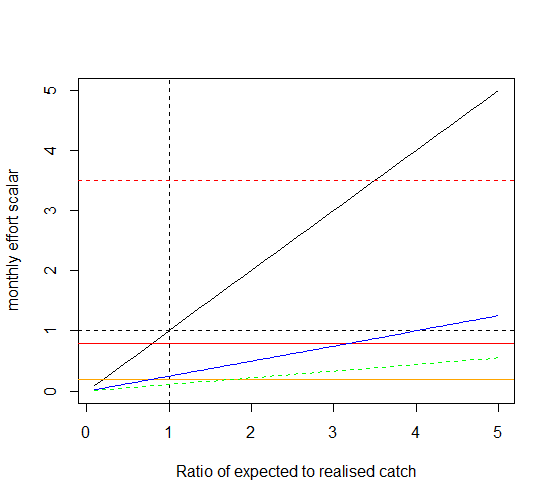
2. Calculate \(\frac{H_{expected,CX,J}}{H_{realised,CX,J}} \cdot \frac{1}{\left( 1 + rank_{CX} \right)^{2}}\) term for each species. This would be a species-specific effort scalar. The graph below shows the effort scalar for a range of expected to realised catch for the highest rank species (rank 0) shown in black, for the second one in blue, and for the third (rank 2) in green dashed line. Remember that in real simulations for each species only one value of the monthly effort scalar will be produced and it will depend on the expected versus realised catch of that species

3. Find the maximum monthly effort scalar across the species. If expected/realised catch < 1 (realised catch is higher than the plan), then the monthly effort scalar is <1 and the effort should be decreased. If the expected versus the realised catch of all species is the same, then the highest ranked species will give the maximum scalar. But the actual values across species will differ, e.g. if the ratio of expected to realised catch of rank 0 species is 1, then its effort scalar is 1. If the expected/realised catch ratio for the second ranked species is 5, then its effort scalar is 1.25. Here Atlantis will take the maximum value across species, i.e. 1.25 in this case.

4. Constrain the minimum effort by the (1-choicebuffer value), where YYY_choicebuffer is the subfleet specific parameter. This parameter defines how quickly a subfleet will downscale the effort if realised catch is higher than expected. In the graph below the red horizontal line corresponds to choicebuffer=0.2 and orange horizontal line corresponds to choicebuffer=0.8.

5. Contrain the maximum effort by the maximum monthly effort Eff_monthly,max which is calculated as

\[Eff_{mothly,max} = monthSc \cdot \left( 1 - downTime_{J} \right) \cdot Nboats_{J}\ \]

Where monthSc is the monthly scalar in the month_scalar global parameter giving a maximum number of days of effort a boat can apply (it can be bigger than 30 if for example one boat has several gears), and downTime_J is the proportion of time a boat from a subfleet J must stay in the port for maintenance given in the YYY_minDownTime parameter. A hypothetical maximum monthly effort limit is shown with a dashed red horizontal line in the graph below.

Figure 12. The monthly effort scalar calculation. See explanation in the text above.

6. Assess whether a subfleet has very high debt levels which will reduce its ability to fish. The tolerable debt levels for each subfleet are set in YYY_TolDebt parameter. If the expected monthly profit from fishing will not increase the debt above the tolerable levels then monthly planned effort is reduced by a proportion set in a global effort_reduction parameter.

17.5.3. Final effort allocations

There are two ways to determine final effort allocations. The baseline model (MultiPlanEffort=1) and Dan Holland model (MultiPlanEffort=0). Here we describe only the baseline multi-plan effort, used in Fulton et al. 2007. The Dan Holland model has been described in Kaplan et al. 2014.

In the baseline model with each new week of the simulation the fishers make the final decision on the temporal and spatial effort allocation (i.e. where to go and how long to fish). This is done based on the updated monthly effort plan, available quota left (if fishing without quota is not allowed and fish_withoutQ=0), and information on spatial CPUE distribution (or value per unit effort or bycatch per unit effort). The calculations are done by the Multi_Plan_Effort_Final_Allocation() in ateconeffort.c

The final effort allocation is done through the following steps:

1. Determine the spatial information about the CPUE values. This is done by calculating the ratio of CPUE in each box by the total CPUE. For these calcualtions the CPUE information of the last month is used (so not the memory period, as applied in other effort models, described in chapter 15).

If value per unit effort information is used (UseVPUE=1) then boxes will be ranked not by CPUE but by VPUE details. Further, if spatial bycatch avoidance is used (SpatialBycatchAvoid=1) then boxes will highest bycatch in the last month will be downscaled.

2. Next, each box is weighted by their mpasc_J,j (MPAYYY parameter from the harvest.prm file, see chapter 16.4), which will change the actual CPUE in this box if some of the box area is closed to fishing. This scaled value is used to calculate the ideal CPUE based effort (CPUE_eff) given the latest CPUE knowledge, monthly effort plan (as explained above) and fisher behavioural flexibility.

\[{CPUEeff}_{J,j} = {mpasc}_{J,j} \cdot Eff_{planned,J,j} \cdot \frac{Flexwgt_{J} \cdot \left( {cpue}_{t,j} - {cpue}_{t - 1,j}\ \right) + {cpue}_{t - 1,j}}{\sum_{j}^{}{cpue}_{J,j}}\]

Where cpue_t,j is the CPUE of subfleet J in the latest memory period t (typically the latest month); and cpue_t-1,j is the CPUE of the subfleet J in the previous memory period (typically a month). The flexwgtJ (YYY_flexweight) parameter reflects how quickly fishers respond to the changing CPUE information – if flexwgt is 1 then effort is based entirely on the latest CPUE data, when flexwgt is 0 then new CPUE information is completely disregarded.

3. Next, the fisher flexibility parameter is used once again to weight the effort matrix, but this time it is not used to assess flexibility to the new CPUE information (old and new CPUE as in the step 2 above), but between the CPUE_eff matrix calculated above (or VPUE, or DisPUE based effort, if appropriate flags are selected) and the monthly effort plan. This means that if fishers are flexible (YYY_flexweight is high or even 1), then the monthly effort plan is entirely overridden by the CPUE information, and if fishers are not flexible (flexweight = 0) they completely follow their monthly effort plan regardless of any information about CPUE.

\[{idEff}_{J,j} = Flexwgt_{J} \cdot \left( {CPUEeff}_{J,j} - Eff_{planned,J} \right) + Eff_{planned,J}\]

4. The ideal spatial idEff effort matrix of subfleet J by box j should further be scaled according to box distance to ports and the scalar determining travel costs of each subfleet FCwgt_J (YYY_FCwgtscale unitless, ranging rom 0 to a very high value) and the variable cost per each subfleet Cost_var,J (YYY_varcost, $/day of effort). This is used to account for the fact that fishers may be unwilling to go to the potentially profitable boxes, if they are too far from the ports. The scaling is done by the sufbleet-box distance matrix DistanceWgt_J,j

\[{DistanceWgt}_{J,j} = \sum_{Z}^{}\frac{Speed_{Y} \cdot dt}{{Z \cdot distance}_{z,j}^{*} \cdot Cost_{var,J}} \cdot FCwgt_{J}\]

where Speed_Y is the speed of the fishery boats, not defined specifically by fisheries but for the entire commercial fisheries (Speed_boat, m hour^-1), dt is the number of hours between the timestep (usually 12, but can be 6 or 24), distance_Z,J is a distance of the subfleet J to port Z, and Z is the total number of ports active for the subfleet J (a port is active if a fishery and subfleet operates from that port and the port is open, see chapter 15.5.9 for a similar case in dynamic fishing effort allocation).

5. Finally, the final effort matrix of subfleet J in each box j is calculated by interpolating between the ideal effort matrix calculated in step 3 versus the effort matrix in the previous step while accounting for boat speed and width of the model domain. This is

\[{finalEff}_{J,j} = {DistanceWgt}_{J,j} \cdot \max\left( 1,\frac{{Speed}_{Y} \cdot dt}{width} \right) \cdot \left( {idEff}_{Y,j} - {oldEff}_{Y,j} \right) + {oldEff}_{Y,j}\]

The (Speed*dt/width) term was explained in the chapter 15.5.8 and simply calculates what distance a fishery Y can travel in one time step compared to the entire model domain (e.g. 0.1 of the maximum possible distance in the model). It shows that if the fishery can cross the entire model domain in one timestep and therefore find itself in any box of the model domain in one timestep, then the scalar will be 1 and the new effort will be the same as the ideal effort. If the scalar is smaller than one, then new effort will be a combination of the old effort and the ideal effort determined above. The DistanceWgt_J,j matrix has been calculated in step 4.

CautionThe role of YYY_flexweight parameter in effort allocation

The YYY_flexweight parameter is used three times in the baseline model (MultiPlanEffort=1) effort allocation and should be carefully considered. It is used to:

1. Update fisher response to latest price and CPUE information when making the annual fishing plan (see chapter 17.5.1).

2. Weight the fisher response to the latest CPUE information (whether to use the latest CPUE data or old CPUE data) – step 2 above.

3. Weight the fisher flexibility in updating the monthly fishing plan with CPUE information (if flexweight=0 then CPUE information is completely ignored and the monthly effort plan is followed) – step 3 above.

Once the effort has been allocation to each box of the model domain, the effort for all subfleets of a fishery is pooled within each box (to get fishery-specific effort per box) and passed to the Harvest submodel.

Table 19. Parameters related to effort allocation

Parameter	Description
MultiPlanEffort	If set to 1, then baseline economic Atlantis model is used to determine effort allocation. If set to 0, the Dan Holland economics model is used (see chapter 17.5.3 for further details).
JanYYYEffort_sub1, FebYYYEffort_sub1, …	Historical average fishing effort (in effort days per box per month) – given for each subfleet of each fishery. This represents a part of the subfleet’s “black books”.
JanCatchXXX_sub1, FebCatchXXX_sub1, …	Historical average catch per species (kg of catch per box per month) – given for each subfleet of each fishery. This represents a part of the subfleet’s “black books”.
JanYYYCPUE_sub1, FebYYYCPUE_sub1, …	Historical average CPUE (kg of catch per one day of effort per box per month) – given for each subfleet of each fishery. This represents a part of the subfleet’s “black books”.
OrigEconCalc	If set to 1 then the expected yearly profit is calculated as earnings minus costs. If set to 0, then profit calculation takes into account CPUE data and proportional contribution of each fish in the catch (see chapter 17.5.1).
TemporalBycatchAvoid	If set to 1, effort planning will take into account monthly historical bycatch and avoid months when bycatch is highest.
SpatialBycatchAvoid	If set to 1, effort planning will take into account spatial historical bycatch and avoid boxes where bycatch is highest.
YYY_flexweight	Parameter setting behavioural flexibility of a subfleet (scalar from 0 to 1). See callout in chapter 17.5.3 for an explanation of how this parameter is used in three different calculations.
YYY_choicebuffer	Parameter (scalar from 0 to 1) setting how quickly a subfleet will update the effort if it deviates from the yearly plan.
UseVPUE	If set to 1, instead of CPUE calculations, Atlantis will use Value per Unit Effort values (which takes into account fish prices at a given time).
YYY_minDownTime	The minimum amount of time (proportion of a month, ranging from 0 to 1) a subfleet must stay in port and therefore cannot fish.
effort_reduction	Global parameter setting a scalar of effort reduction that a subfleet will experience if its debt is higher than the value given in the YYY_TolDebt parameter.
YYY_FCwgtscale	Scalar (from 0 to a very high value) that will affect the willingness of a subfleet to travel to distant boxes.
YYY_varcost	Cost of fishing per subfleet per day ($ / effort_day).